Pasha Zavari

Studies in Chaos and Finance: Chapter IV

April 29, 2025 Pasha ZavariLeave a comment

In this chapter we will use the conditional representations in (32) and (42) to calculate the first statistical moment, the mean. The diffusion integral in (29) can be re-written as:

$\sum_ {i = 1}^{n} \sum_ {j = 1}^{n} \Sigma^{-1}_{ij} \begin{cases} W_t^{\{i\}, 2} \frac {e^{\alpha_{ii} t}}{\alpha_{ii}} - \frac {2}{\alpha_{ii}} \int_0^t W_s^{\{i\}} e^{\alpha_{ii} s} \, dW_s^{\{i\}} + \frac {1 - e^{\alpha_{ii} t}}{\alpha_{ii}^2}, & \text{if } i = j \\ \frac{1}{\alpha_{ij}} e^{\alpha_{ij} t} W_t^{\{i\}} W_t^{\{j\}} - \frac{1}{\alpha_{ij}} \int_0^t e^{\alpha_{ij} s} \left[ W_s^{\{i\}}\, dW_s^{\{j\}} + W_s^{\{j\}}\, dW_s^{\{i\}} \right] - \delta_{ij} \frac{e^{\alpha_{ij} t} - 1}{\alpha_{ij}^2}, & \text{if } i \ne j \end{cases}$ $(43)$

The expectation under $i = j$ can be derived as follows:

$\begin{aligned} & = \langle W_t^{\{i\}, 2} \frac {e^{\alpha_{ii} t}}{\alpha_{ii}} \rangle - \langle \frac {2}{\alpha_{ii}} \int_0^t W_s^{\{i\}} e^{\alpha_{ii} s} \, dW_s^{\{i\}} \rangle + \langle \frac {1 - e^{\alpha_{ii} t}}{\alpha_{ii}^2} \rangle \\ & = \langle W_t^{\{i\}, 2} \rangle \frac {e^{\alpha_{ii} t}}{\alpha_{ii}} - \frac {2}{\alpha_{ii}} \int_0^t \langle W_s^{\{i\}} e^{\alpha_{ii} s} \rangle \, dW_s^{\{i\}} + \langle \frac {1 - e^{\alpha_{ii}t}}{\alpha_{ii}^2} \rangle \\ & = \langle W_t^{\{i\}, 2} \rangle \frac {e^{\alpha_{ii} t}}{\alpha_{ii}} - \frac {2}{\alpha_{ii}} \int_0^t \underbrace {\langle W_s^{\{i\}} \rangle }_{= \, 0} e^{\alpha_{ii} s} \, dW_s^{\{i\}} + \langle \frac {1 - e^{\alpha_{ii} t}}{\alpha_{ii}^2} \rangle \\ & = \frac{t e^{\alpha_{ii} t}}{\alpha_{ii}} + \frac{1 - e^{\alpha_{ii} t}}{\alpha_{ii}^2} \end{aligned}$ $(44)$

where we can interchange expectation and integration in the second step by Fubini’s theorem. The expectation under $i \neq j$ is a little more nuanced and will require more wrangling. Recall the definition of covariace between two non-overlapping processes:

$Cov(W_t^{i}, W_t^{j}) = \langle W_t^{i} W_t^{j} \rangle - \langle W_t^{i} \rangle \langle W_t^{j} \rangle$ $(45)$

We know that $\langle W_t^{i} \rangle \langle W_t^{j} \rangle = 0$ and that using the Quadratic Covariation we can show:

$Cov(W_t^{i}, W_t^{j}) = \langle W_t^{i} W_t^{j} \rangle = \rho_{ij} \sqrt{Var(W_t^{i}) Var(W_t^{j})} = \rho_{ij} \sqrt{t^2}$ $(46)$

The expectation under $i \neq j$ in (49) can be expressed as:

$\frac{e^{\alpha_{ij} t}}{\alpha_{ij}} \langle W_t^{\{i\}} W_t^{\{j\}} \rangle - \frac{1}{\alpha_{ij}} \int_0^t e^{\alpha_{ij} s} \left[ \langle W_s^{\{i\}} \rangle\, dW_s^{\{j\}} + \langle W_s^{\{j\}} \rangle\, dW_s^{\{i\}} \right] - \langle \delta_{ij} \frac{e^{\alpha_{ij} t} - 1}{\alpha_{ij}^2} \rangle$ $(47)$

Following the results where $\langle W_s^{\{i\}} \rangle = \langle W_s^{\{j\}} \rangle = 0$ and $\langle \delta_{ij} \rangle = \rho_{ij}$ our expression in (47) simplifies to:

$\rho_{ij} \left( \frac{t e^{\alpha_{ij} t}}{\alpha_{ij}} + \frac{1 - e^{\alpha_{ij} t}}{\alpha_{ij}^2} \right)$ $(48)$

Interestingly, the only noted difference between $i = j$ and $i \neq j$ is the correlation term $\rho_{ij}$ . Therefore, the expectation of the diffusion integral in (29) is given by:

$\langle \int_0^t \boldsymbol{W}_s^T (e^{\textbf{A} s} \circ \Sigma^{-1}) \boldsymbol{W}_s \, ds \, \rangle = \sum_ {i = 1}^{n} \sum_ {j = 1}^{n} \Sigma^{-1}_{ij} \left(\frac{t e^{\alpha_{ij} t}}{\alpha_{ij}} + \frac{1 - e^{\alpha_{ij} t}}{\alpha_{ij}^2} \right) \times \begin{cases} 1, & \text{if } i = j \\ \rho_{ij}, & \text{if } i \ne j \end{cases}$ $(49)$

Model Assumptions

April 16, 2025 Pasha ZavariLeave a comment

The modeling decision to employ $f(\sigma W)$ rather than a time-varying correlation matrix reflects a deliberate trade-off between expressive power and analytical tractability. The function $f$ is used to capture nonlinear heteroskedastic behavior influenced by interaction between multiple stochastic systems. More Specifically:

Nonlinearity: The transformation via f permits the introduction of local, nonlinear distortion effects that are challenging to capture using purely linear correlation structures.
Parsimony: A full time-evolving correlation matrix introduces a significant number of parameters, which can lead to identifiability issues, particularly when empirical data is limited.
Interpretability: The function f offers a modular and interpretable way to model external influence on endogenous noise, aligning with methods used in stochastic volatility modeling.

The choice here is intentional and consistent with the goal of modeling systems where volatility is driven by nonlinear interaction rather than simply nonstationary correlation.

The differential form introduced as Equation (7) in the paper is given by:

$df(\mathbf{X}) = \sum_{k = 1}^{n} \frac{\partial f(\mathbf{X})}{\partial x_k} \, dx_k. \nonumber$

This expression implies that $f$ is differentiable and locally homogeneous of degree 1, satisfying:

$f(\lambda \mathbf{x}) = \lambda f(\mathbf{x}), \quad \text{for any } \lambda \in \mathbb{R}, \mathbf{x} \in \mathbb{R}^n. \nonumber$

This is not an assumption of global homogeneity, but rather a local property that ensures consistency under scalar transformation. The rationale behind this is twofold:

Stability Under Scaling: Systems influenced by proportional shocks should exhibit consistent variance scaling properties under time evolution.
Differentiability: The form of df ensures that perturbations to each dimension of X yield tractable expressions in the stochastic differential system.

This framework is particularly useful for modeling multiplicative noise processes or systems with volatility clustering.

Equation (6) as originally written,

$dx^{i,j}_t = \alpha x^{i,j}_t dt + f(\sigma W^{\{i,j\}}_t), \nonumber$

is shorthand for a more general formulation in which the driving noise $W^{\{i,j\}}_t$ is a linear combination of two Wiener processes:

$\tilde{W}_t = \lambda_1 W^i_t + \lambda_2 W^j_t, \quad \lambda_1, \lambda_2 \in \mathbb{R}. \nonumber$

The resulting system becomes:

$dx_t = \alpha x_t dt + f(\sigma \tilde{W}_t). \nonumber$

This construction acknowledges that real-world systems are rarely closed and often subject to external influences that do not respect strict orthogonality. The function $f$ absorbs these dependencies into a nonlinear transformation of noise.

Given that $f \neq 0$ , the resulting process is no longer a Levy process in the strict sense. The introduction of $f$ breaks both stationary increment and independent increment properties, depending on its form. This departure is intentional, as the goal is to model a more physically realistic, heteroskedastic process where the variance is no longer constant and memory effects may emerge. The nonlinear properties of $f(W(\boldsymbol{z}))$ described in Chapter II, which can be thought of as a type of memory function, arise from its intrinsic dependence on past values of $W_t$ . This means that for some integer-time stochastic process $\{Z_n; n \geqslant 1\}$ , our model may satisfy one of two conditions:

A $\textbf{Submartingale}$ condition:

$\mathbb{E}[|Z_n|] < \infty, \quad \mathbb{E}[Z_n | Z_{n-1}, Z_{n-2}, \dots, Z_1] \geq Z_{n-1}, \quad n \geq 1, \nonumber$

or a $\textbf{Supermartingale}$ condition:

$\mathbb{E}[|Z_n|] < \infty, \quad \mathbb{E}[Z_n | Z_{n-1}, Z_{n-2}, \dots, Z_1] \leq Z_{n-1}, \quad n \geq 1. \nonumber$

Studies in Chaos and Finance: Chapter III

April 5, 2025April 26, 2025 Pasha ZavariLeave a comment

The nonlinear properties of $f(W(\boldsymbol{z}))$ described in Chapter II, which can be thought of a type of memory function, arise from its intrinsic dependence on past values of $W_t$ . This means that for some integer-time stochastic process $\{Z_n; n \geqslant 1\}$ our model satisfies one of two relations: a Submartingale defined by

$\begin{aligned} \mathsf{E} [|Z_n|]<\infty; \quad \mathsf{E}[Z_n|Z_{n-1},Z_{n-2},...,Z_1] \geq Z_{n-1} ;\quad n \geq 1 \nonumber \end{aligned}$ $(29)$

or a Supermartinagle defined by

$\begin{aligned} \mathsf{E}[|Z_n|] <\infty; \quad \mathsf{E}[Z_n|Z_{n-1},Z_{n-1},...,Z_1]\leq Z_{n-1};\quad n \geq 1 \nonumber \end{aligned}$ $(30)$

The focus of this chapter will be to explore the fundamental stochastic characteristics of (28) using the above defintions. To begin, it will help to re-write the integral using summation nation:

$\int_0^t \boldsymbol{W}_s^T (e^{\textbf{A} s} \circ \Sigma^{-1}) \boldsymbol{W}_s \, ds \, \equiv \sum_ {i = 1}^{n} \sum_ {j = 1}^{n} \Sigma^{-1}_{ij} \int_0^t e^{\alpha_{ij} s} W_s^{\{i\}} W_s^{\{j\}} \, ds$ $(31)$

Note that when $i = j$ we have $W_s^{\{j\}, 2}$ .

In order to address these non-deterministic integrals in (31) we will need to apply Itô’s Lemma expressed as

$f(t,W_t) - f(0,0) = \int_0^t \frac{\partial f}{\partial t}(s,W_s) \, ds + \int_0^t \frac{\partial f}{\partial x}(s,W_s) \, dW_s + \frac{1}{2}\int_0^t \frac{\partial^2 f}{\partial x^2}(s,W_s) \, ds$ $(32)$

For $i = j$ we have

$\begin{aligned} f(t, W_t^{i}) - f(0, 0) & = \frac {1}{\alpha_{ii}} [W_s^{\{i\}, 2} e^{\alpha_{ii} s}]_{0}^{t} \\ \int_0^t \frac{\partial f}{\partial t}(s,W_s^{\{i\}}) \, ds & = \int_0^t W_s^{\{i\}, 2} e^{\alpha_{ii} s} \, ds \\ \int_0^t \frac{\partial f}{\partial x}(s,W_s^{\{i\}}) \, dW_s^{\{i\}} & = \frac {2}{\alpha_{ii}} \int_0^t W_s^{\{i\}} \, e^{\alpha_{ii} s} \, dW_s^{\{i\}} \\ \frac{1}{2}\int_0^t \frac{\partial^2 f}{\partial x^2}(s,W_s^{\{i\}}) \, ds & = \frac {1}{\alpha_{ii}} \int_0^t e^{\alpha_{ii} s} \, d_s \end{aligned}$ $(33)$

which yields

$\begin{aligned} \int_0^t W_s^{\{i\}, 2} e^{\alpha_{ii} s} \, ds & = W_t^{\{i\}, 2} \frac {e^{\alpha_{ii} t}}{\alpha_{ii}} - \frac {2}{\alpha_{ii}} \int_0^t W_s^{\{i\}} e^{\alpha_{ii} s} \, dW_s^{\{i\}} - \frac {1}{\alpha_{ii}} \int_0^t e^{\alpha_{ii} s} \, d_s \\ & = W_t^{\{i\}, 2} \frac {e^{\alpha_{ii} t}}{\alpha_{ii}} - \frac {2}{\alpha} \int_0^t W_s^{\{i\}} e^{\alpha_{ii} s} \, dW_s^{\{i\}} + \frac {1 - e^{\alpha_{ii} t}}{\alpha_{ii}^2} \end{aligned}$ $(34)$

The case $i \neq j$ will require a little more mathematical machinery. The first step is to re-write the integral using Itô’s Differential:

$d(xy)_{t} = x_{t}dy_{t} + y_{t}dx_{t} + dx_{t}dy_{t}, \quad dx_{t}dy_{t} = d[x,y]_{t}$ $(35)$

The quadratic covariation denoted by $[x,y]_{t}$ underpins a critical difference between classical calculus and stochastic calculus. This topic is quite involved and, for the sake of brevity, will be skipped in this chapter. I plan to return to it in the future with a comprehensive overview. Continuing on, we know that using Itô’s multiplication table we can deduce that $dx_{t}dy_{t} = \delta_{ij} s$ , where $\delta_{ij}$ is the Kronecker delta and where $\delta_{ij} = 1$ when $i = j$ . The expression can then be re-written as

$d(W_s^{\{i\}} W_s^{\{j\}}) = W_s^{\{i\}}\, dW_s^{\{j\}} + W_s^{\{j\}}\, dW_s^{\{i\}} + \delta_{ij}\, ds$ $(36)$

Applying Itô’s product rule to:

$Y_s = e^{\alpha_{ij} s} W_s^{\{i\}} W_s^{\{j\}}$ $(37)$

we can derive:

$\begin{aligned} dY_s & = \alpha_{ij} e^{\alpha_{ij} s} W_s^{\{i\}} W_s^{\{j\}}\, ds + e^{\alpha_{ij} s}\, d(W_s^{\{i\}} W_s^{\{j\}}) \\ & = \alpha_{ij} e^{\alpha_{ij} s} W_s^{\{i\}} W_s^{\{j\}}\, ds + e^{\alpha_{ij} s} \left[ W_s^{\{i\}}\, dW_s^{\{j\}} + W_s^{\{j\}}\, dW_s^{\{i\}} + \delta_{ij}\, ds \right] \end{aligned}$ $(38)$

Integrating both sides in (36):

$Y_t = Y_0 + \int_0^t \alpha_{ij} e^{\alpha_{ij} s} W_s^{\{i\}} W_s^{\{j\}}\, ds + \int_0^t e^{\alpha_{ij} s} \left[ W_s^{\{i\}}\, dW_s^{\{j\}} + W_s^{\{j\}}\, dW_s^{\{i\}} \right] + \delta_{ij} \int_0^t e^{\alpha_{ij} s}\, ds$ $(39)$

Since ${W_0^{\{i\}} = W_0^{\{j\}} = 0 }$ , we have ${Y_0 = 0 }$ , so:

$e^{\alpha_{ij} t} W_t^{\{i\}} W_t^{\{j\}} = \alpha_{ij} \int_0^t e^{\alpha_{ij} s} W_s^{\{i\}} W_s^{\{j\}}\, ds + \int_0^t e^{\alpha_{ij} s} \left[ W_s^{\{i\}}\, dW_s^{\{j\}} + W_s^{\{j\}}\, dW_s^{\{i\}} \right] + \delta_{ij} \int_0^t e^{\alpha_{ij} s}\, ds$ $(40)$

Rearranging (38) and solving for $I_t = \int_0^t e^{\alpha_{ij} s} W_s^{\{i\}} W_s^{\{j\}}\, ds$ :

$\alpha I_t = e^{\alpha_{ij} t} W_t^{\{i\}} W_t^{\{j\}} - \int_0^t e^{\alpha_{ij} s} \left[ W_s^{\{i\}}\, dW_s^{\{j\}} + W_s^{\{j\}}\, dW_s^{\{i\}} \right] - \delta_{ij} \int_0^t e^{\alpha_{ij} s}\, ds$ $(41)$

Provided that $\alpha_{ij} \neq 0$ , we can isolate $I_t$ :

$I_t = \frac{1}{\alpha_{ij}} e^{\alpha_{ij} t} W_t^{\{i\}} W_t^{\{j\}} - \frac{1}{\alpha_{ij}} \int_0^t e^{\alpha_{ij}s} \left[ W_s^{\{i\}}\, dW_s^{\{j\}} + W_s^{\{j\}}\, dW_s^{\{i\}} \right] - \frac{\delta_{ij}}{\alpha_{ij}} \int_0^t e^{\alpha_{ij} s}\, ds$ $(42)$

Given that the closed form solution to $\int_0^t e^{\alpha_{ij} s}\, ds = \frac{e^{\alpha_{ij} t} - 1}{\alpha_{ij}}$ , we can also write:

$\frac{\delta_{ij}}{\alpha_{ij}} \int_0^t e^{\alpha_{ij} s}\, ds = \delta_{ij} \frac{e^{\alpha_{ij} t} - 1}{\alpha_{ij}^2}$ $(43)$

Finally we have:

$\int_0^t e^{\alpha_{ij} s} W_s^{\{i\}} W_s^{\{j\}}\, ds = \frac{1}{\alpha_{ij}} e^{\alpha_{ij} t} W_t^{\{i\}} W_t^{\{j\}} - \frac{1}{\alpha_{ij}} \int_0^t e^{\alpha_{ij} s} \left[ W_s^{\{i\}}\, dW_s^{\{j\}} + W_s^{\{j\}}\, dW_s^{\{i\}} \right] - \delta_{ij} \frac{e^{\alpha_{ij} t} - 1}{\alpha_{ij}^2}$ $(44)$

Studies in Chaos and Finance: Chapter II

March 20, 2025April 29, 2025 Pasha ZavariLeave a comment

In the previous chapter we proposed the Ornstein-Uhlenbeck process as the foundation for our stochastic model:

$dx^{i,j}_t = \alpha x^{i,j}_tdt + \tilde{W}(z_i, z_j)$ $(18)$

The results derived in (16) follow a special case of state variables $x$ and $y$ expressed in terms of standard normal variables $z_1$ and $z_2$ . Using the Cholesky decomposition of a covariance matrix $\Sigma$ :

$\Sigma = \textbf{L} \textbf{L}^{T}$ $(19)$

we can show that

$\Sigma = \begin{bmatrix} \sigma_{1} & 0 \\ 0 & \sigma_{2} \end{bmatrix} \begin{bmatrix} 1 & \rho \\ \rho & 1 \end{bmatrix} \begin{bmatrix} \sigma_{1} & 0 \\ 0 & \sigma_{2} \end{bmatrix} \\ = \begin{bmatrix} l_{11} & 0 \\ l_{21} & l_{22} \end{bmatrix} \begin{bmatrix} l_{11} & l_{12} \\ 0 & l_{22} \end{bmatrix}.$ $(20)$

Solving for $L$ we get:

$l_{11} = 1, \indent l_{21} = \rho, \indent l_{22} = \sqrt{1 - \rho^2}$ $(21)$

Now we can express these variables in terms of $L$ and the standard normal variables:

$\begin{aligned} x &= \sigma_1 l_{11} z_1 = \sigma_1 z_1 \\ y &= \sigma_1 (l_{21} z_1 + l_{22} z_2) = \sigma_2 (\rho z_1 + \sqrt{1 - \rho^2} z_2) \end{aligned}$ $(22)$

matching the stated forms in (12) and (13). The result in (22) will be applied in its general form when solving the n-state extension of our SDE in (18). It will help to rearrange the expression into its proper differential form with an additional term, $\boldsymbol{\mu}$ , to account for the rate at which our stochastic process changes with time

$\dot{\textbf{x}}(t) + \textbf{A} (\textbf{x}(t) - \boldsymbol{\mu}) = \tilde{W}(\mathbf{z})$ $(23)$

where,

$\frac{\partial {\textbf{x}}(t)}{\partial t} = \begin{bmatrix} \frac{\partial x_1(t)}{\partial t} \\ \frac{\partial x_2(t)}{\partial t} \\ \vdots \\ \frac{\partial x_i(t)}{\partial t} \end{bmatrix}, \indent \textbf{A} = \begin{bmatrix} \alpha_{11} & \alpha_{12} & \cdots & \alpha_{1j} \\ \alpha_{21} & \alpha_{22} & \cdots & \alpha_{2j} \\ \vdots & \vdots & \ddots & \vdots \\ \alpha_{i1} & \alpha_{i2} & \cdots & \alpha_{ij} \\ \end{bmatrix}, \indent \boldsymbol{\mu} = \begin{bmatrix} \mu_{11} \\ \mu_{21} \\ \vdots \\ \mu_{i1} \end{bmatrix}.$ $(24)$

Note that $\textbf{A}$ is an upper triangle matrix:

$\textbf{A}_{ij} = \begin{cases} a_{ij}, & \text{if } i \leq j \\ 0, & \text{if } i > j \end{cases}$ $(25)$

This is what is known as a Linear First Order Inhomogeneous Stochastic Differential Equation with function coefficients written as

$\frac {\partial x(t)}{\partial t} + P(t) x(t) = Q(t)$ $(26)$

and can be solved by its general solution

$e^{-\int_ {\:}^{t} P(t) \, dt} \left[ {\int_ {\:}^{t} e^{\int_ {\:}^{\lambda} P(\epsilon) \, d\epsilon} Q(\lambda)\, d\lambda} + t_0 \right]$ $(27)$

where $e^{\int_ {\:}^{t} P(t) \, dt}$ is the integrating factor. Plugging (18) into our solution we have

$\begin{aligned} \textbf{x}(t) = \boldsymbol{x_0} e^{-\textbf{A} t} + \boldsymbol{\mu} (\textbf{I} - e^{-\textbf{A} t}) - e^{-\textbf{A} t} \int_0^t \boldsymbol{W}_s^T (e^{\textbf{A} s} \circ \Sigma^{-1}) \boldsymbol{W}_s \, ds \\ \end{aligned}$ $(28)$

given $\boldsymbol{x_0} \in \mathbb{R}^{n \times 1}, A \in \mathbb{R}^{n \times n}, \boldsymbol{\mu} \in \mathbb{R}^{n \times 1}$ and identity matrix $I \in \mathbb{R}^{n \times n}$ . The deterministic part of the (28) is rather trivial. In order to address the non-deterministic integrands, however, requires working knowledge of Itô Calculus. In the next chapter we will lay out the logic to make sense of these integrals.

Studies in Chaos and Finance: Chapter I

March 14, 2025April 29, 2025 Pasha ZavariLeave a comment

A mathematician is a device for turning coffee into theorems – Alfréd Rényi

One of the notable limitations of a standard autoregressive model is that it intrinsically assumes distributive homogeneity across the historical time horizon. A system’s impulse response to a change in the value of a shock term, $k$ , at some time-step, $t_{n - i}$ , must also account for influences imposed by external systems evolving in parallel – specially if there exist a correlation known to be of particular significance. These nuanced characteristics of real-world scenarios further complicate an autoregressive model’s broad application as a time-varying forecast. This new series explores mathematical machinery borrowed from Itô calculus as a means to derive a systematic solution to an n-state autoregressive model where significant correlation exists between two interacting time-varying processes with underlying random components.

Imagine a singular stationary point in a closed system. An infinitesimally small region containing within it maximum information in a state of equiprobability. In a state of such rigid order the propensity for information mobility is minimized. Now consider allowing this system to interact with another time-varying process. The structural stability of our information space due to volatility from information gain, deteriorates as its entropy increases. This process is accelerated as our system evolves forward in time.

Suppose that the entropic state for the subset of initial information $S_i$ , observed at time $t_n$ , is bound by the preceding entropic state at time $t_{n-1}$ . Therefore, in the case of discrete intervals we have

$x_t = \alpha x_{t-1}+z_t$ $(1)$

where $\alpha$ is a scale parameter and $z_t$ represents white noise. Rearranging the terms in (1) we can show

$(1-\alpha) x_t+\alpha\nabla x_t = z_t$ $(2)$

This result derives from the fact that the first difference of a random walk forms a purely random process. The analogous interpretation of (2) in continuous time can be described by the general form

$\alpha x(t)+\frac {\partial x(t)}{\partial t} = z(t)$ $(3)$

This expression is what is commonly called a first-order continuous autoregressive equation CAR(1). A CAR process of order $p$ is generally represented by the following equation

$x^p(t)+\alpha_{p-1}x^{p-1}(t)+...+\alpha_0x(t) = z(t)$ $(4)$

Note that $z(t)$ represents a continuous white noise process which cannot physically exist. We will instead replace this term with one that represents small infinitesimal changes characterized by Gaussian orthogonal increments. That is to say that for any two non-overlapping time intervals $\left\{t_a, t_b\right\}$ and $\left\{t_c, t_d\right\}$ the increments $W^d_{t}-W^c_{t}$ are independent of past values $W^b_{t}-W^a_{t}$ . Furthermore, $W_0$ is always zero. $W_t$ is described as pure a Wiener process. We will rewrite (3) in its first-order stochastic differential form

$dx_t = \alpha x_tdt + \sigma dW_t$ $(5)$

where $\alpha$ and $\sigma$ are more formally referred to as drift and volatility. Expression (5) appears in the well known Ornstein-Uhlenbeck model. It is, however, an incomplete characterization of our particular chaotic system. This is because our information space is no longer a closed system, rather one that is interacting with another chaotic system with a systematic influence on the state variable $x(t)$ . As a result of this, the variability of distribution throughout time is no longer constant. Our system is said to be heteroskedastic. In order to account for this non-linearity we can relax orthogonality by introducing a function $f$ that describes the relationship between these interacting systems

$dx^{i,j}_t = \alpha x^{i,j}_tdt + f(\sigma W^{\{i,j\}}_t)$ $(6)$

Let us define a $\tilde{W}$ that is some linear combination of our closed system, $W^i_t$ , and the outside system, $W^j_t$ . We can formalize this interpretation by writing out the total differential form

$df(\textbf{X}) = \sum_ {k = 1}^{n} \frac {\partial f(\textbf{X})}{\partial x_k} \, dx_k$ $(7)$

which can be re-written as

$\int df(\textbf{X}) = \idotsint_S \, \sum_ {k = 1}^{n} \frac {\partial f(\textbf{X})}{\partial x_k} \, dx_i \quad dx_1 \dots dx_n$ $(8)$

Now lets assume that

$\frac {\partial f(\textbf{X})}{\partial x_k} = z_k$ $(9)$

which implies

$\int d\tilde{W}(\textbf{Z}) = \idotsint_S \, \sum_ {k = 1}^{n} z_k \, dz_k \quad dz_1 \dots dz_n$ $(10)$

where $\tilde{W}(\textbf{Z}) \mapsto f(\textbf{X})$ . For $n = 2$ the above expression reduces to

$\tilde{W}(z_i, z_j) = \frac{1}{2} (z_i^2 + z_j^2)$ $(11)$

assuming zero constants of integration and where $z_i$ and $z_j$ are independent $\mathcal{N} \sim (0, t)$ . Based on this we can define the following

$W^{\{i\}}_t = \sigma_i z_i$ $(12)$

$W^{\{j\}}_t = \sigma_j (\rho z_i + \sqrt{1 - \rho^{2}} z_j)$ $(13)$

where $\rho \in \{-1, 1\}$ and $W^{\{j\}}_t$ describes the interaction between stochastic systems $i$ and $j$ . Solving for $z_i$ and $z_j$ we have

$z_i = \frac {1}{\sigma_1} \, W^{\{i\}}_t$ $(14)$

$z_j = \frac {\sigma_i W^{\{j\}}_t - \rho \sigma_j W^{\{i\}}_t}{\sigma_i \sigma_j \sqrt{1 - \rho^2}}$ $(15)$

Therefore, it follows

$\begin{aligned} \tilde{W}(z_i, z_j) & = \frac {1}{2} [\frac {1}{\sigma_i} \, W^{\{i\},2}_t + (\frac {\sigma_i W^{\{j\}}_t - \rho \sigma_j W^{\{i\}}_t}{\sigma_i \sigma_j \sqrt{1 - \rho^2}})^2] \\ & = - \frac {1}{2(1 - \rho^2)} [\frac {W^{\{i\},2}_t}{\sigma_i^2} + \frac{W^{\{j\},2}_t}{\sigma_j^2} - 2 \rho \frac {W^{\{i\}}_t W^{\{j\}}_t}{\sigma_i \sigma_j}] \end{aligned}$ $(16)$

Given the result above, we can re-write (6)

$dx^{i,j}_t = \alpha x^{i,j}_tdt + \tilde{W}(z_i, z_j)$ $(17)$

In the next chapter we will outline the steps that solve for $x(t)$ , extending these results to derive an n-state CAR framework.

Riemann’s Zeta and Random Walks

June 7, 2018March 14, 2025 Pasha ZavariLeave a comment

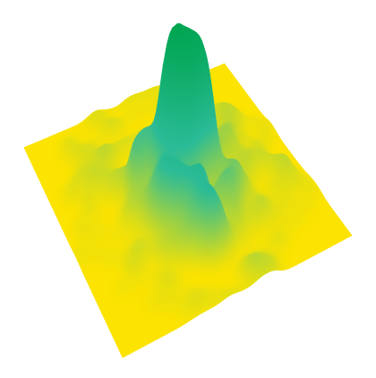
The Riemann Zeta function is a function of a complex variable $s$ that analytically continues the sum of the Dirichlet series

$\zeta(s) = \sum\limits_{n=1}^{\infty} \frac{1}{n^s}$

In 1737, the revered Swiss mathematician, Leonhard Euler, discovered the fundamental connection between the Zeta function and prime numbers. The proof is as follows, given

$\zeta (s)=\sum\limits _{n=1}^{\infty }{\frac {1}{n^{s}}} = 1+{\frac {1}{2^{s}}}+{\frac {1}{3^{s}}}+{\frac {1}{4^{s}}}+{\frac {1}{5^{s}}}+\ldots$ $(1.1)$

we will multiply both sides of the equation by ${\frac {1}{2^{s}}}$

${\frac {1}{2^{s}}}\zeta (s) = {\frac {1}{2^{s}}}+{\frac {1}{4^{s}}}+{\frac {1}{6^{s}}}+{\frac {1}{8^{s}}}+{\frac {1}{10^{s}}}+\ldots$ $(1.2)$

then subtract $(1.2)$ from $(1.1)$ to remove all factors of 2

$\left(1-{\frac {1}{2^{s}}}\right)\zeta (s)=1+{\frac {1}{3^{s}}}+{\frac {1}{5^{s}}}+{\frac {1}{7^{s}}}+{\frac {1}{9^{s}}}+{\frac {1}{11^{s}}}+{\frac {1}{13^{s}}}+\ldots$

Repeating this for factors of 3

$\frac {1}{3^{s}}\left(1-{\frac {1}{2^{s}}}\right)\zeta (s) = {\frac {1}{3^{s}}}+{\frac {1}{9^{s}}}+{\frac {1}{15^{s}}}+{\frac {1}{21^{s}}}+{\frac {1}{27^{s}}}+{\frac {1}{33^{s}}}+\ldots$

$\left(1-{\frac {1}{3^{s}}}\right)\left(1-{\frac {1}{2^{s}}}\right)\zeta (s)=1+{\frac {1}{5^{s}}}+{\frac {1}{7^{s}}}+{\frac {1}{11^{s}}}+{\frac {1}{13^{s}}}+{\frac {1}{17^{s}}}+\ldots$

and so on. If we continue this process to infinity for $\frac{1}{p^s}$ , where $p$ is a prime, the expression reduces to

$\ldots \left(1-{\frac {1}{11^{s}}}\right)\left(1-{\frac {1}{7^{s}}}\right)\left(1-{\frac {1}{5^{s}}}\right)\left(1-{\frac {1}{3^{s}}}\right)\left(1-{\frac {1}{2^{s}}}\right)\zeta (s) = 1$

which can be rearranged to produce

$\zeta(s) = \frac{1}{\left(1-{\frac {1}{2^{s}}}\right)\left(1-{\frac {1}{3^{s}}}\right)\left(1-{\frac {1}{5^{s}}}\right)\left(1-{\frac {1}{7^{s}}}\right)\left(1-{\frac {1}{11^{s}}}\right)+\ldots } = \prod\limits_{\forall p\:\in\:\mathrm{P}}^{\:} \frac{1}{1-p^{-s}}$ $(1.3)$

So why are we doing all of this? Well, it turns out the reciprocal of the Zeta function has some remarkable properties of its own.

Consider the inverse based on Euler’s prime product formula

$\frac{1}{\zeta(s)} = \prod\limits_{\forall p\:\in\:\mathrm{P}}^{\:} \left(1-p^{-s}\right) = \left(1-\frac{1}{2^s}\right)\left(1-\frac{1}{3^s}\right)\left(1-\frac{1}{5^s}\right)\ldots$

expanding this expression we have

$\frac{1}{\zeta(s)} = 1 + \sum_{n \text{ prime}} \left({\frac{-1} {n^s} }\right) + \sum_{n \mathop = p_1 p_2} \left({ \frac{-1}{p_1^s} \frac{-1} {p_2^s} }\right) + \sum_{n \mathop = p_1 p_2 p_3} \left({ \frac {-1} {p_1^s} \frac {-1} {p_2^s} \frac{-1}{p_3^s} }\right) + \ldots$

which can be rearranged to demonstrate

$\frac{1}{\zeta(s)} = 1 + \frac{-1}{2^s} + \frac{-1}{3^s} + \frac{0}{4^s} + \frac{-1}{5^s} + \frac{1}{6^s} + \frac{-1}{7^s} + \frac{0}{8^s} + \frac{0}{9^s} + \frac{1}{10^s} + \frac{-1}{11^s} + \ldots$ $(1.4)$

On close examination one can see that the numerator in $(1.4)$ actually corresponds to the values of the Möbius function $\mu(x)$ . Indeed, the reciprocal of the Zeta function can be formally defined by